Revolving credit facility
Throughout the model build process, we have set up our model to react in a way that pre-supposed we are before the transaction date. If we change the tariff and resolve the model, we’ll get a different IRR and debt amount. We are sculpting the ratios to hit a specific DSCR target.
In this section, the final substantive piece of modelling in the book, we’re looking at how we can change the model to analyse changes after the transaction date.
In reality, once the asset is in operation, we already have a debt structure in place and are committed to certain debt repayments. We can’t go back in history to change these.
Let’s say we’re looking at a situation where we have some unexpected maintenance costs that we didn’t foresee when we first modelled the project. If we add these to the model now, the debt amount and repayment profile will change when we re-solve the model. But in reality, that couldn’t happen after the debt has been drawn.
So in this chapter, we’re going to look at the following:
- How to set the model up to look at “post-financial close scenarios” - where the debt amount and the repayment profile are fixed.
- What will the impact be of unexpected additional maintenance costs?
- How might we finance those costs with a revolving credit facility?
The solution for this bonus chapter is available in the file pack you'll receive when you purchase the handbook. See file 4.62 FMH rcf BEG 01a.
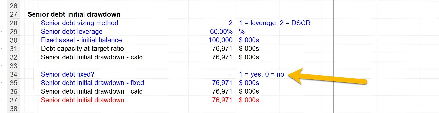
Fixing our debt package
If assumptions change after the debt package has been fixed and the debt drawn, the debt amount and repayments will no longer be changeable.
I’ve therefore included those items in the solve sheet set-up. This way, we can store a “hard-coded” copy of the key debt line items.
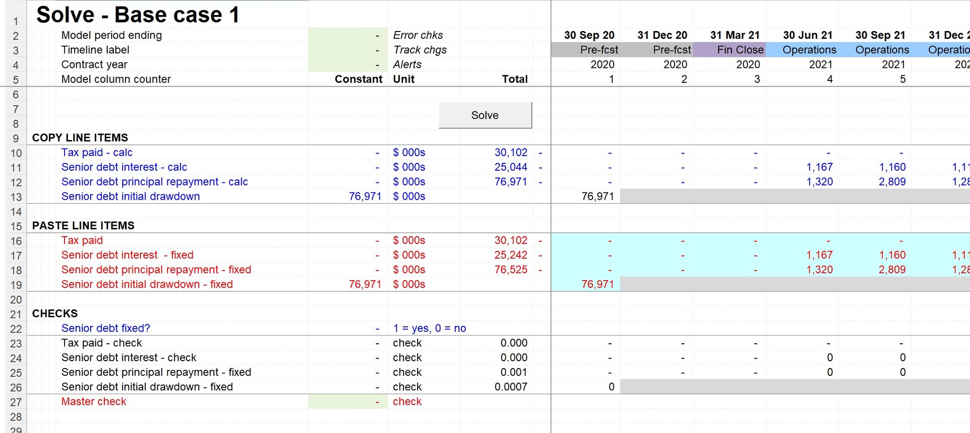
I’ve added a switch to allow us to run the model with the debt fixed.
When this switch is active, the senior debt calculation will pick up the stored values from the solve sheet. When the switch is inactive, the model will use the calculated amounts.
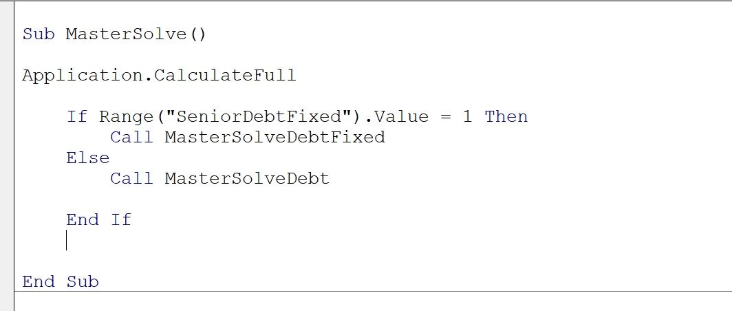
This also requires a change to our solving macro.
When running the model in “fixed debt” mode, the calculated debt capacity and repayment lines will differ from the stored values. But we don’t want the model to overwrite the stored values. But we still want the tax line to be solved to deal with the circularity in the model.
Therefore I’ve updated the VBA to operate differently depending on whether the debt is fixed. If the debt is fixed, only the tax line will be solved. If the debt is not fixed, all the lines will be iterated, and therefore a new hard-coded version of the debt repayment profile will be stored.
Hit Alt+F11 in the reference file to look at the new code.
The MasterSolve macro now looks at whether the debt is fixed and runs a different solve macro if it is.
Let’s test this.
I start with a model showing the same output as before:
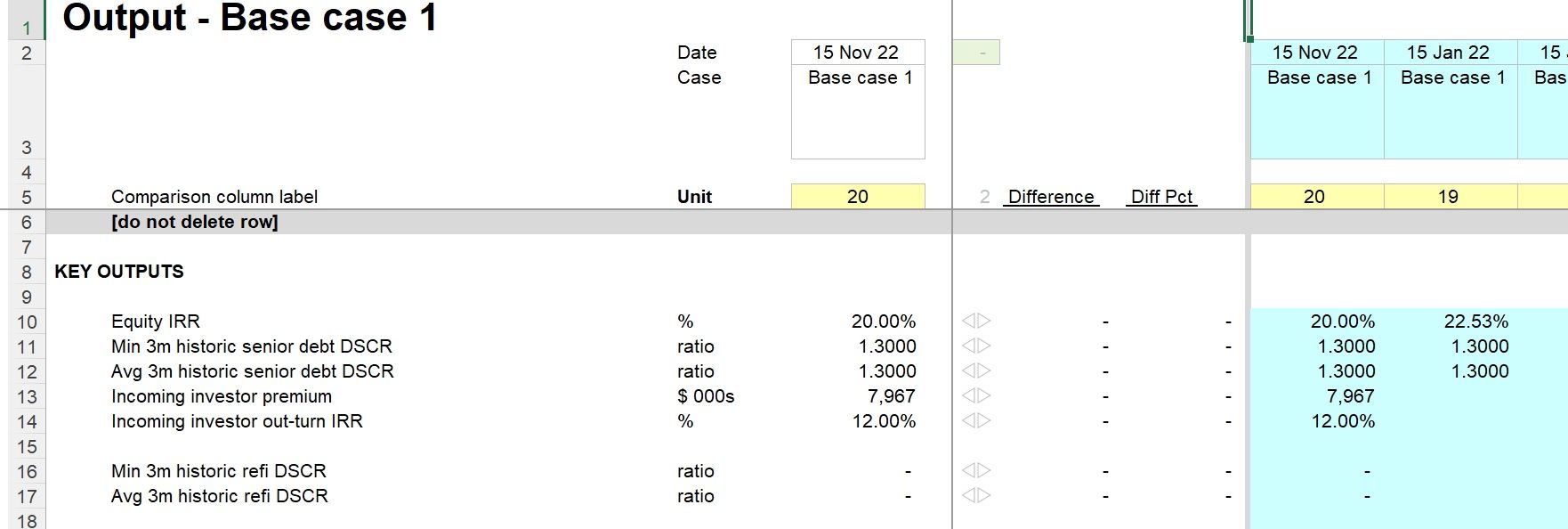
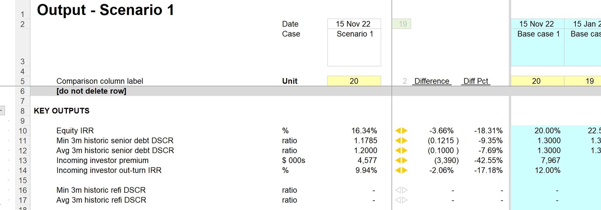
My starting model has been solved with a 6.5c tariff. What do we expect to see if we fix the debt and reduce the tariff? I’d be expecting to see a lower IRR and lower coverage ratios. The debt should no longer be resized to meet our DSCR target, so I’d expect ratios lower than the 1.30 we used to size the debt.
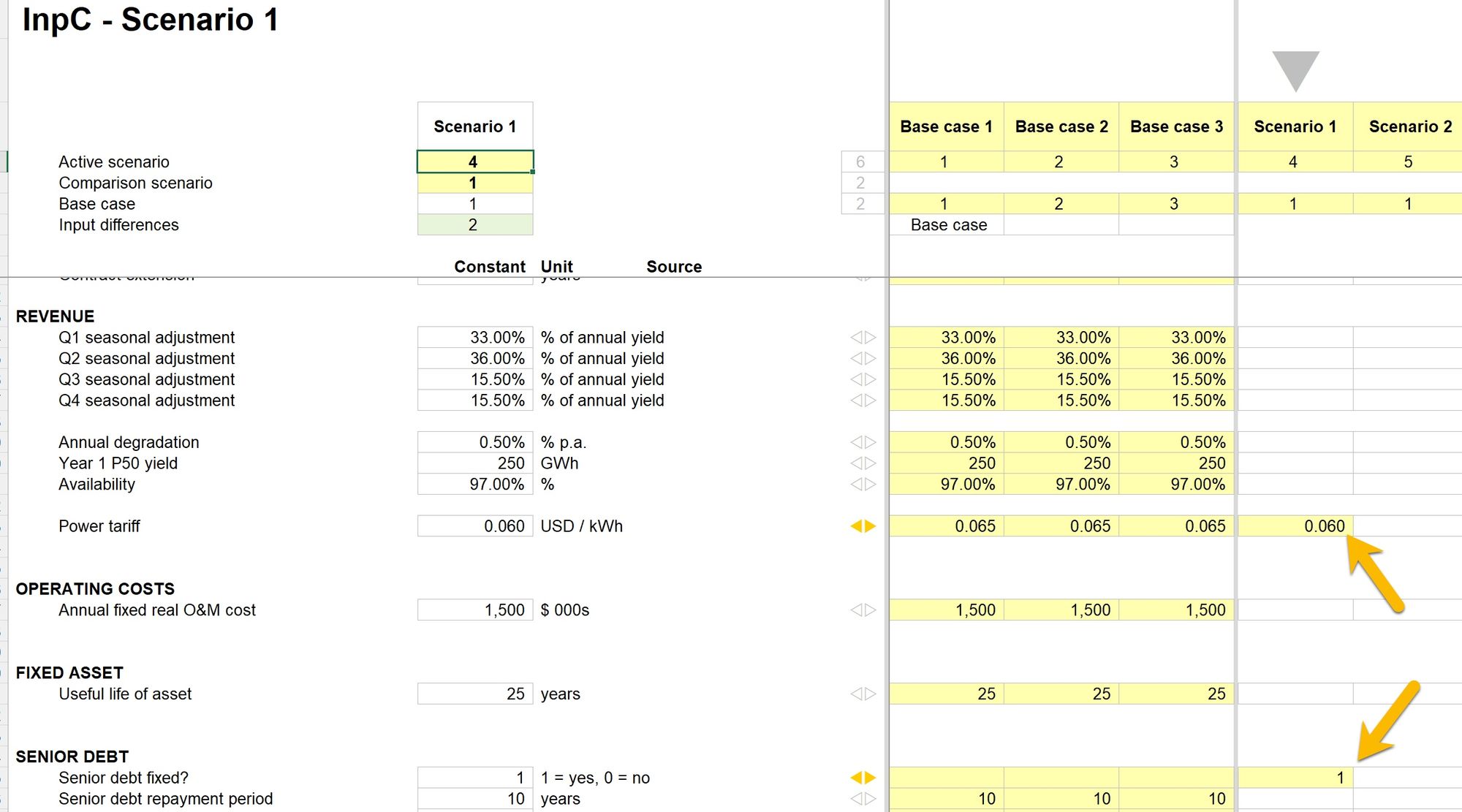
If I solve the model in “fixed debt” mode, the debt does not resize, the repayments don’t change, and I see a lower IRR and lower coverage ratios.
If I change the tariff back to what it was before and re-solve the model with the debt still fixed, I should get the same outputs as before; since the stored debt profile was saved in this scenario.
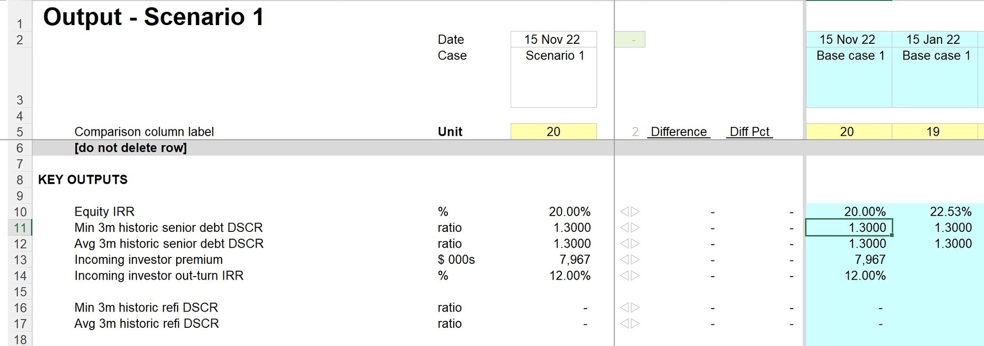
This all is working as expected.
Unexpected maintenance costs
I’ve added an InpS sheet to look at the impact of maintenance costs. This kind of sheet is useful for adding inputs that are profiled over time.
I’ve put in two amounts of $2m. These are just hypothetical numbers so that we can look at the impact and understand how to model in this scenario.
If I solve the model in Fixed debt mode with these additional costs, I’m seeing a lower IRR and breached coverage ratios.
I also see a negative cash balance on my balance sheet. What’s happening here?
There isn’t enough cash to pay for those costs, so the model is “assuming” a free overdraft is in place to pay for them. In reality, this is understating the impact of these costs; we’d need to be able to put in place some financing to cover them.
Revolving credit facility
A Revolving Credit Facility or “RCF” is much like an overdraft facility. It’s a facility that can be drawn when required and repaid when cash is available.
We will use this to meet the temporary cash shortfall caused by the additional maintenance costs.
To model the RCF, we need the following sections:
- RCF drawdown - we need to know when there are cash shortfalls to be funded by the RCF
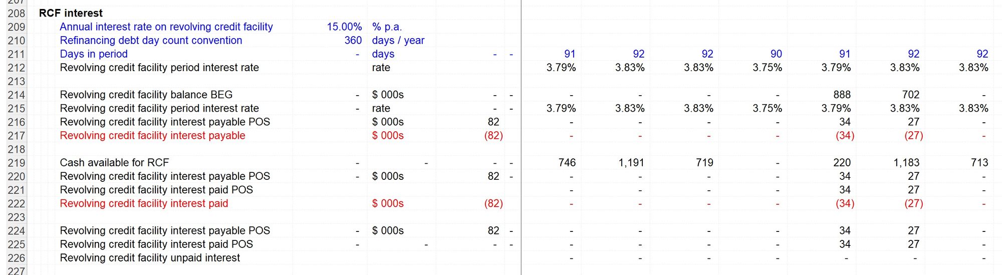
- RCF interest costs - we need to model the interest and know what to do if there isn’t enough cash to pay the interest. In this case, any unpaid interest will be added to the outstanding balance of the facility and paid later.
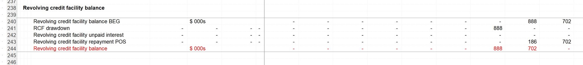
- RCF repayment - since the RCF debt is expensive, we’ll want to pay off the balance as quickly as possible.
Let’s look at each of these sections in the model.
RCF drawdown
As we’ve seen in several other areas of the model, we are “testing the amount of cash” by taking the cash beginning balance and adding the relevant cash flow line from the cash waterfall.
This case is slightly different. If the number is positive, cash is available to repay the RCF. If it’s negative, we need to draw down on the RCF. I’m splitting the line into two - the positive one showing the cash available and the negative one becoming the RCF drawdown.
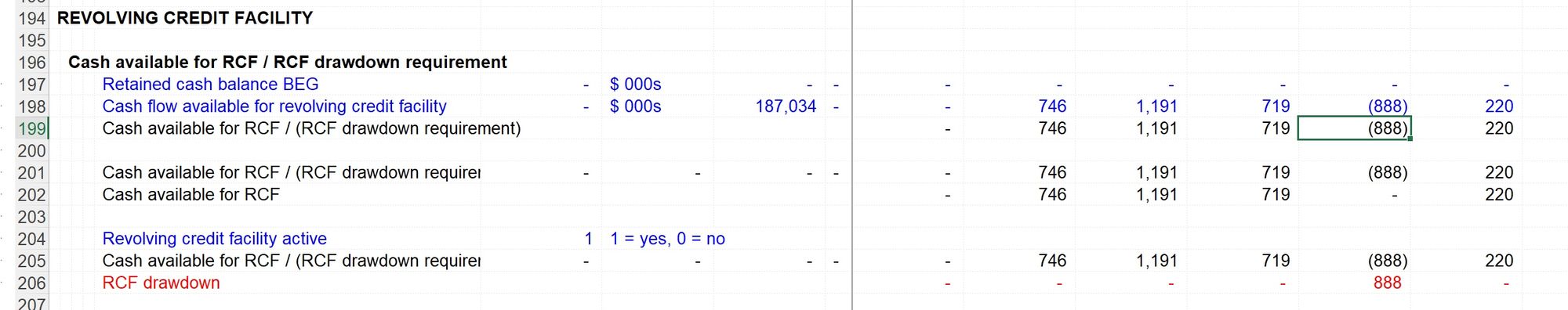
The drawdown line goes to our cash flow statement and the balance corkscrew for the RCF facility.
RCF interest costs
There are several stages to this calculation:
- What interest is payable? This looks at the balance outstanding on the RCF and the RCF interest rate. This is the same as we have used in other places.
- What interest can be paid? For this, we are looking at the cash available and comparing it against the interest payable. The lower of those tells us how much interest can be paid.
- The interest payable goes to the income statement. The interest paid goes to the cash flow statement.
- We then subtract the interest paid from the interest payable to give us the interest that cannot be paid. This is added to the RCF balance.
RCF repayment
Again there are several stages.
- We subtract the interest paid from the cash available. This tells us how much cash is remaining to make a repayment after interest has been paid.
- We compare this against the amount of RCF outstanding. We pay the lower of cash available after interest has been paid, and the RCF balance due.
- The repayment line goes to the cash flow statement and flows into the balance corkscrew to reduce the outstanding RCF balance.
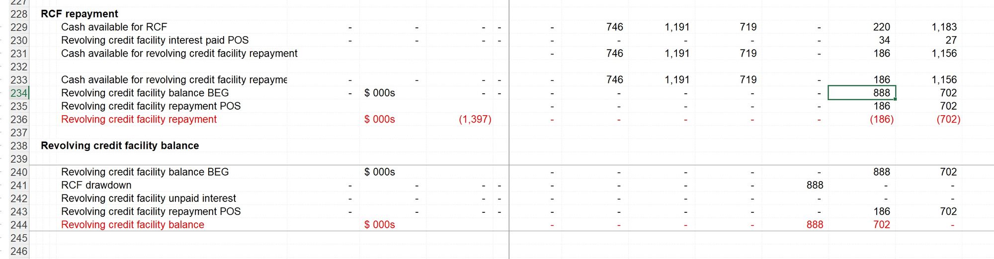
When we look at our financial statements now, we are no longer showing the “unauthorised overdraft” that we had before. Instead, we are drawing on the RCF to meet the cash shortfall and showing the RCF balance increase.
This calculation structure can be replicated in any model when you need to add an RCF.
The solution for this bonus chapter is available in the file pack you'll receive when you purchase the handbook. See file 4.62 FMH rcf END 01a.

Comments
Sign in or become a Financial Modelling Handbook member to join the conversation.
Just enter your email below to get a log in link.