How to analyse model differences using Variance tabs
The output sheet helps analyse and understand differences between model runs at a high level. Sometimes, however, we need to see how differences change over time, in more detail, and on specific line items that may not even be on our output sheet.
For example, let's say we use the sample model from this chapter to test the impact of changing from sculpted to straight-line debt repayment.
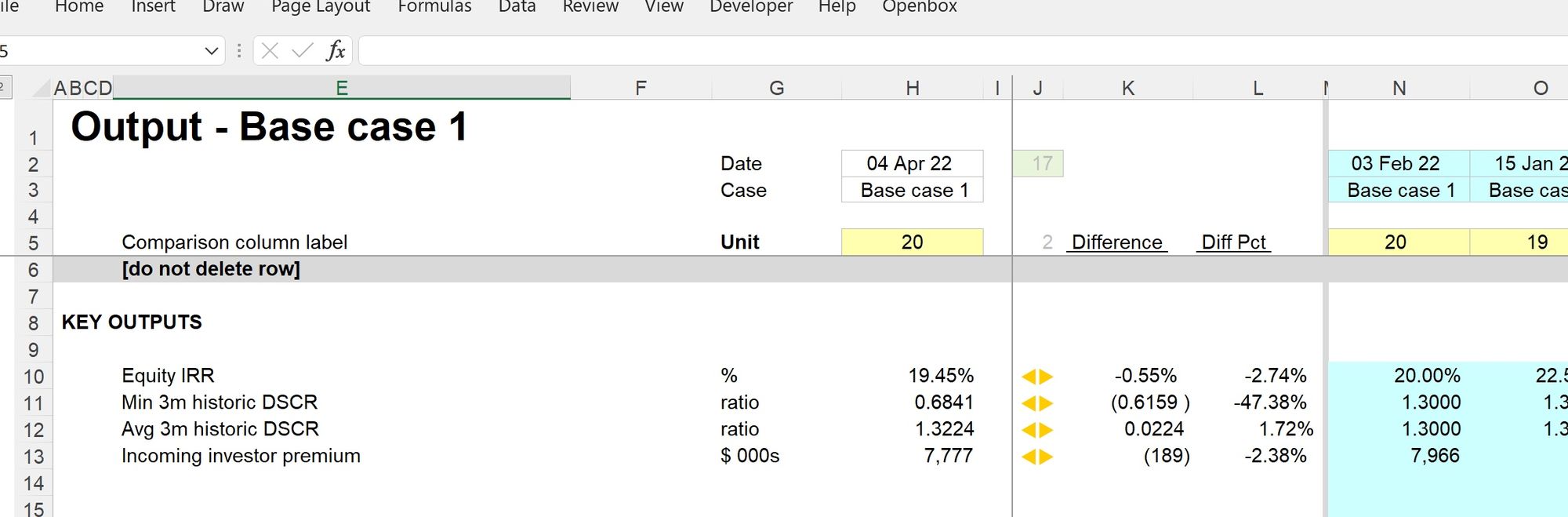
The output sheet tells us that the IRR will reduce by 55 bps. This is valuable information, but often we need more detail to understand why output numbers are changing.
The variance tabs can help us with this kind of analysis.
To obtain the worked example file to accompany this chapter buy the financial modelling handbook.
How to use the variance tabs
1. Run the model in the "start case". In our model, that's the case with sculpted debt repayment.
It's worth ensuring that you have an output track saved in this case so that you can also compare differences at a high level.
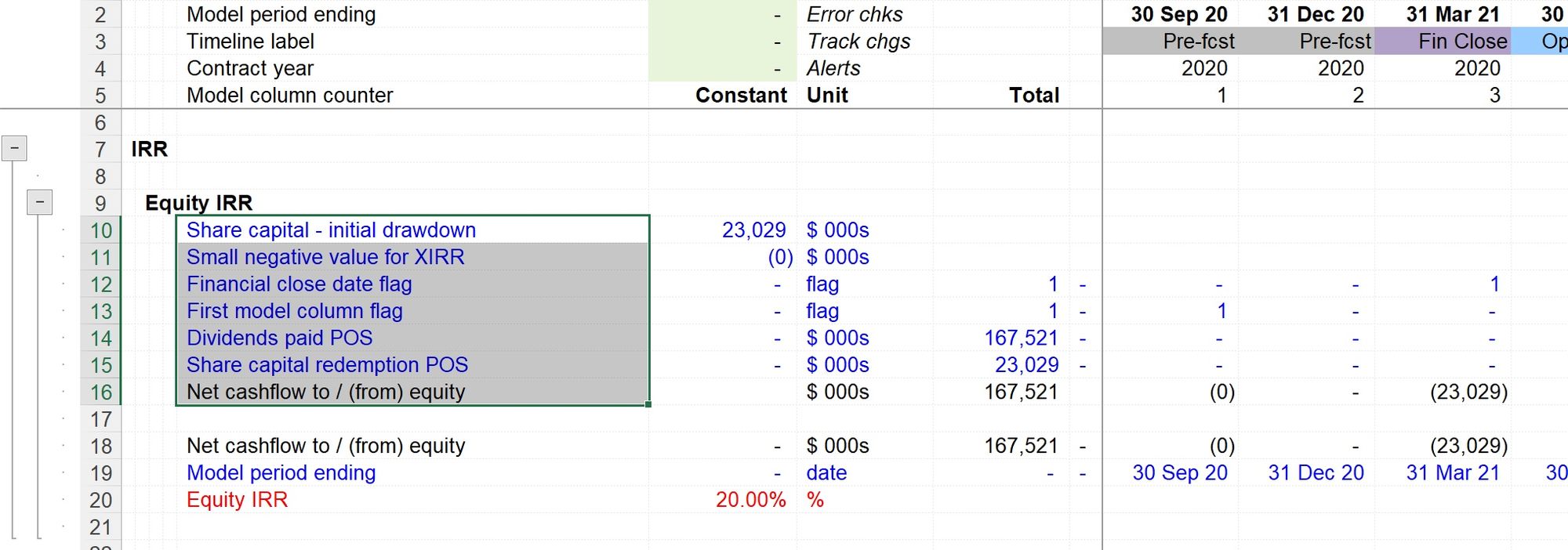
2. Select the rows you want to analyse in more detail to understand the delta caused by the input or scenario change.
In our case, we want to examine the impact on the shareholder cashflows.
3 Run the Variance tabs macro
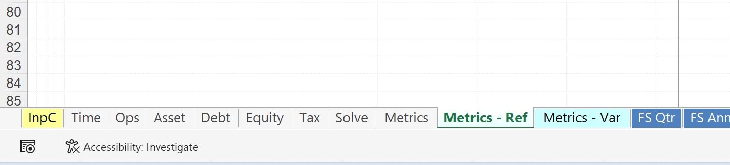
Two new sheets will be added to your model. Each will carry the original sheet name, plus a suffix:
Ref - this contains a hard-coded copy of the lines you selected at the previous step. Similar to the way the output sheet works, this provides our reference data for the model as it currently is.
Var - this contains a calculation comparing the "live" line items you initially selected with the hard-coded Ref version.
4 Change to the scenario you wish to compare.
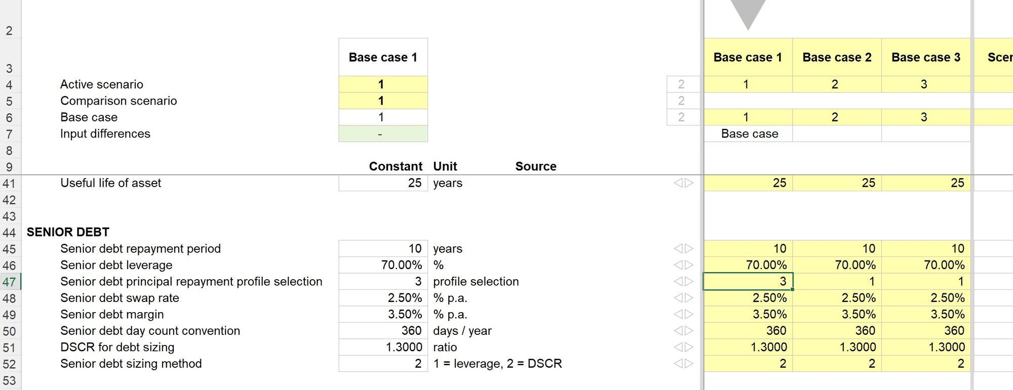
In our case, we want to switch to straight-line debt repayment, which we do on the Input sheet in row 47
Once we recalculate or resolve the model, the Ref sheet shows how our selected rows have changed.
Importantly we can see these changes over time. It provides valuable additional analytical data to help us better understand the output changes.
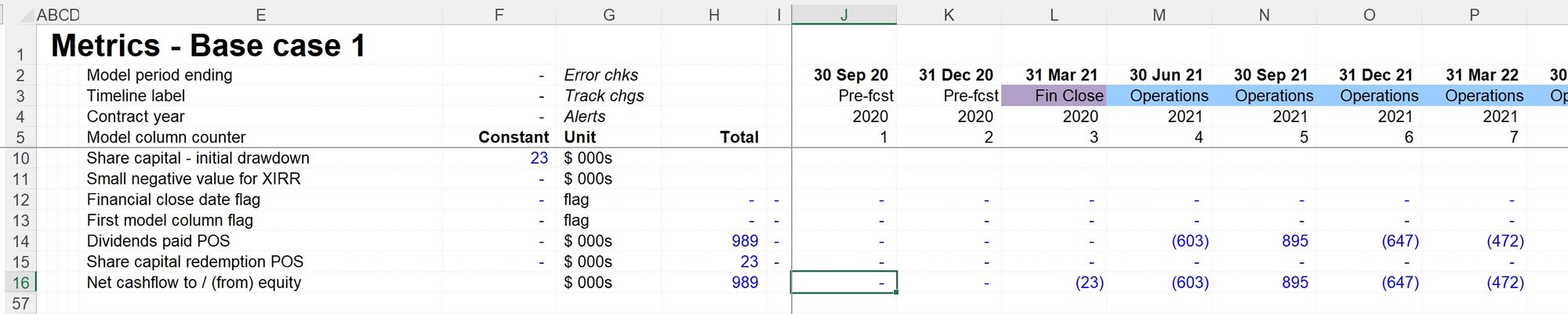
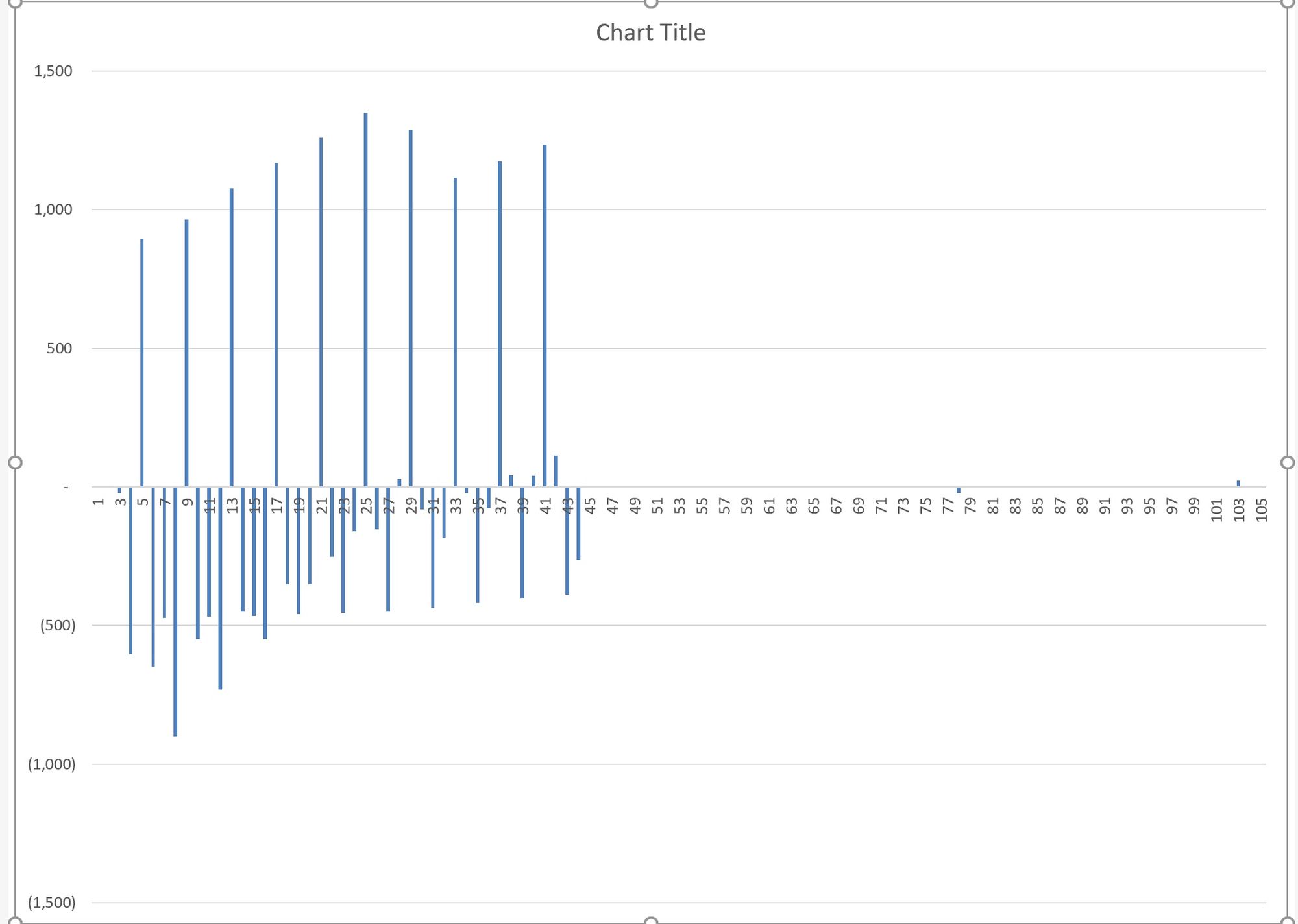
It can be helpful to chart these changes. For example, the profile of equity cashflow differences due to the change in debt sculpting looks like this:
We can also do additional analysis using the calculated delta lines. For example, it can be helpful when looking at equity cashflows to look at the cumulative differences over time:
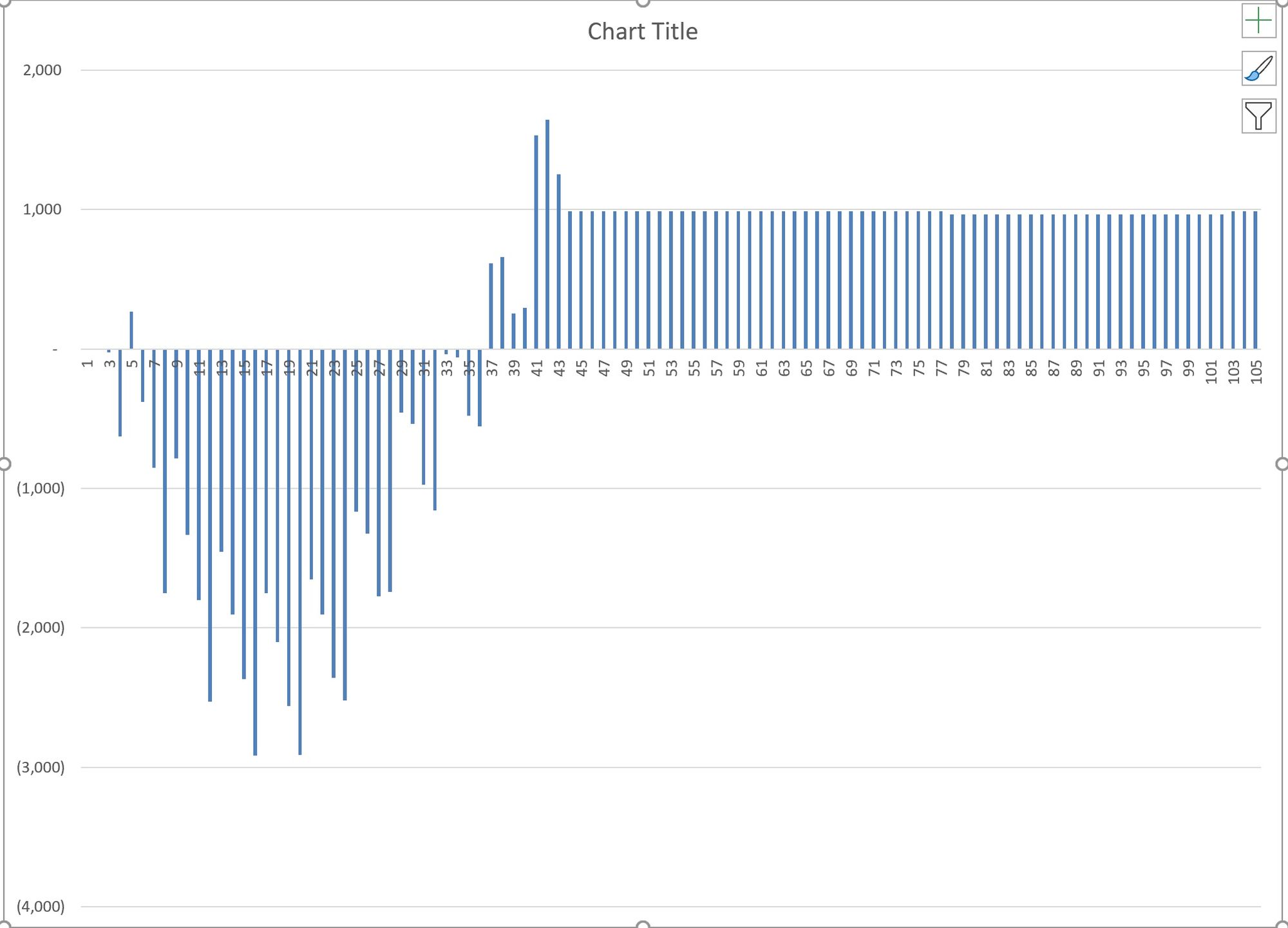
In this case, we can see that while total dividends are higher when we apply straight-line debt repayment, the cumulatively equity cashflows are lower in the early periods. This paints a much clearer explanatory picture of why the IRR is lower with straight-line debt repayment.
The variance tabs are handy for testing our explanatory hypotheses about changes in the model.
Download the end file for this section:
To obtain the worked example file to accompany this chapter buy the financial modelling handbook.

Comments
Sign in or become a Financial Modelling Handbook member to join the conversation.
Just enter your email below to get a log in link.