Debt modelling 5: Debt service coverage ratio
All lenders seek to understand and quantify the ability of the borrower to repay their debt.
Download the lesson start file:
To obtain the worked example file to accompany this chapter buy the financial modelling handbook.
For mortgages, lenders will apply a maximum loan to value ratio to ensure that home buyers also have sufficient "equity" in the home. They will also apply a multiple of borrowers earnings to determine the affordability of the mortgage.
It's not dissimilar in a business like this.
The "loan to value" ratio in this instance is given by the maximum leverage that lenders are willing to see in the business. Lenders will determine the "affordability" using a Debt Service Coverage Ratio, or DSCR.
DSCR is defined as Cash flow Available for Debt Service / Debt Service.
There can be different time periods that this ratio can be calculated over. The ratio is also sometimes forward-looking, sometimes backwards looking.
It measures the ratio of cash available to pay debt to the debt due.
Typically lenders will look at both the minimum and average values of the ratio. Average DSCR can sometimes be defined as the average of the periodic ratios, or it can be total CFADS over the term of the debt, dividend by the total debt service.
Modelling this ratio is relatively straightforward as we already have the ingredients from previous work that we've done.
We will calculate the three-month historic DSCR.
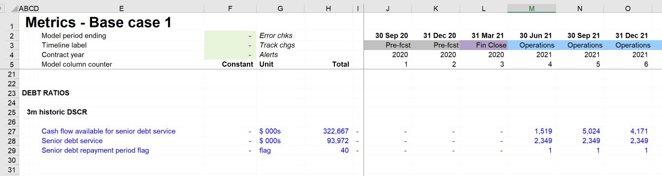
Step 1: Gather your ingredients.
You need:
- Cash flow available for debt service (from the cash flow statement)
- Debt service (we have already added this to our debt sheet
- Senior debt repayment period flag.
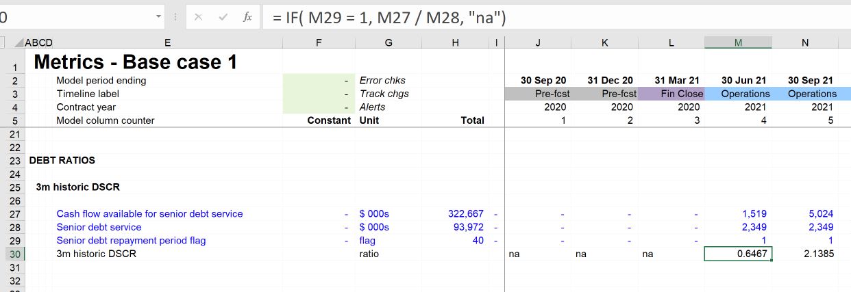
Step 2: Calculate the period ratio.
It's helpful in this calculation to use an IF statement referring to the flag. If it's not a ratio calculation date, the IF statement returns "na" rather than zero. When we calculate the minimum and average ratios, the periods in which there is no ratio will be ignored by the MIN and AVERAGE functions.
Step 3: Calculate the minimum ratio and the average of the periodic ratios
Using the MIN and AVERAGE functions.
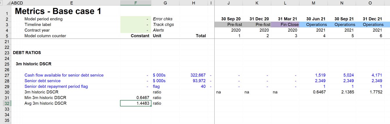
We can see that the minimum ratio is below 1. This is another way of observing what we have already seen; in the first period, there is not enough cash flow to make the debt service payments due in that period.
If we chart the 3m DSCR, we can see a wide seasonal swing, reflecting the high seasonality in revenues.
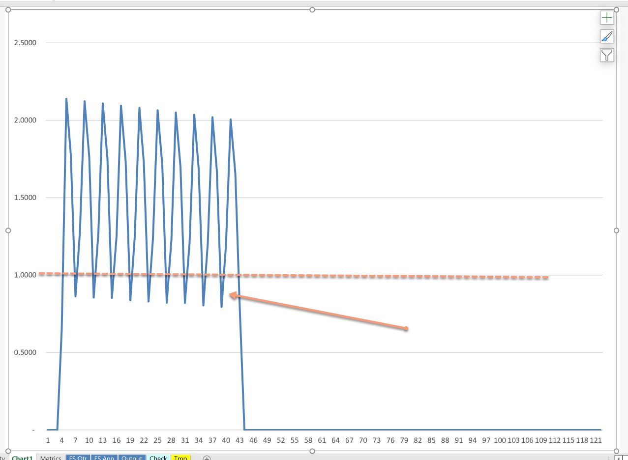
We can see that the ratio falls below 1 in multiple periods. This means that the business does not have sufficient cash to pay debt in these periods. This is not a base case that project sponsors could present to lenders.
The average ratio is relatively healthy, though, and within the range of what would be required on a project like this. We will see in the next chapter how we can use the ratio to calculate the debt capacity of the business and profile debt service to ensure that we always meet the minimum cover ratio requirement.
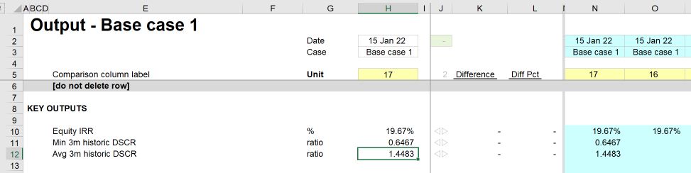
Step 4: Add the ratios to the output sheet.
Using skill 12, link the ratios to the Output sheet so that we can continue to track them as we have been doing our IRR. These are critical metrics for lenders, and we want to ensure we keep an eye on them.
Download the model completed to this point:
To obtain the worked example file to accompany this chapter buy the financial modelling handbook.

Comments
Sign in or become a Financial Modelling Handbook member to join the conversation.
Just enter your email below to get a log in link.